Data exploration with KQL externaldata
In my day job, I spend a lot of time querying and analysing vast amounts of security data to find interesting patterns and prototype detections.
Azure Data Explorer (ADX), originally known as Kusto, is an
incredible platform for achieving this with its rich Kusto Query Language (KQL) - and
is the real engine behind Microsoft’s Security business.
Whilst ADX is designed for ingesting, indexing and querying data, it’s also pretty good at performing ad-hoc analysis on data held in Azure Storage blobs or Amazon S3 buckets - including GitHub repos. Note that arbitrary websites are unlikely to work, but uploading to GitHub is usually a pretty simple procedure.
I thought it could be useful to provide a few examples of this - using the externaldata KQL operator, which dynamically fetches and parses data from external storage into a temporary ADX table.
externaldata to retrieve Seaborn Iris Dataset
A basic externaldata KQL query is self-contained. It must be executed against a cluster and database (everything in ADX requires this),
but it doesn’t depend on or use any real tables - so any cluster/database will do.
The following KQL query loads the Iris dataset from Seaborn as CSV, and parses this into an ADX table:
externaldata(sepal_length:real, sepal_width:real, petal_length:real, petal_width:real, species:string) [
    "https://raw.githubusercontent.com/mwaskom/seaborn-data/master/iris.csv"
]
with(format='csv', ignoreFirstRecord=true)
Running this will output the full table. Note that we need to tell ADX how to parse the data and convert and type the columns correctly. See the externaldata docs for full details.
Basic Analysis
Given the conversion, we can start to perform some simple analysis and plot some summary statistics.
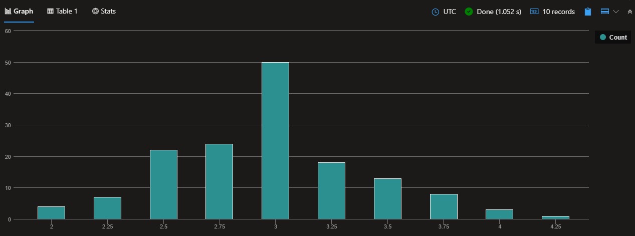
The following query counts the number of samples with sepal widths bucketed by 0.25cm:
externaldata(sepal_length:real, sepal_width:real, petal_length:real, petal_width:real, species:string) [
    "https://raw.githubusercontent.com/mwaskom/seaborn-data/master/iris.csv"
]
with(format='csv', ignoreFirstRecord=true)
| summarize Count = count() by sepal_width = bin(sepal_width, 0.25)
| render columnchart
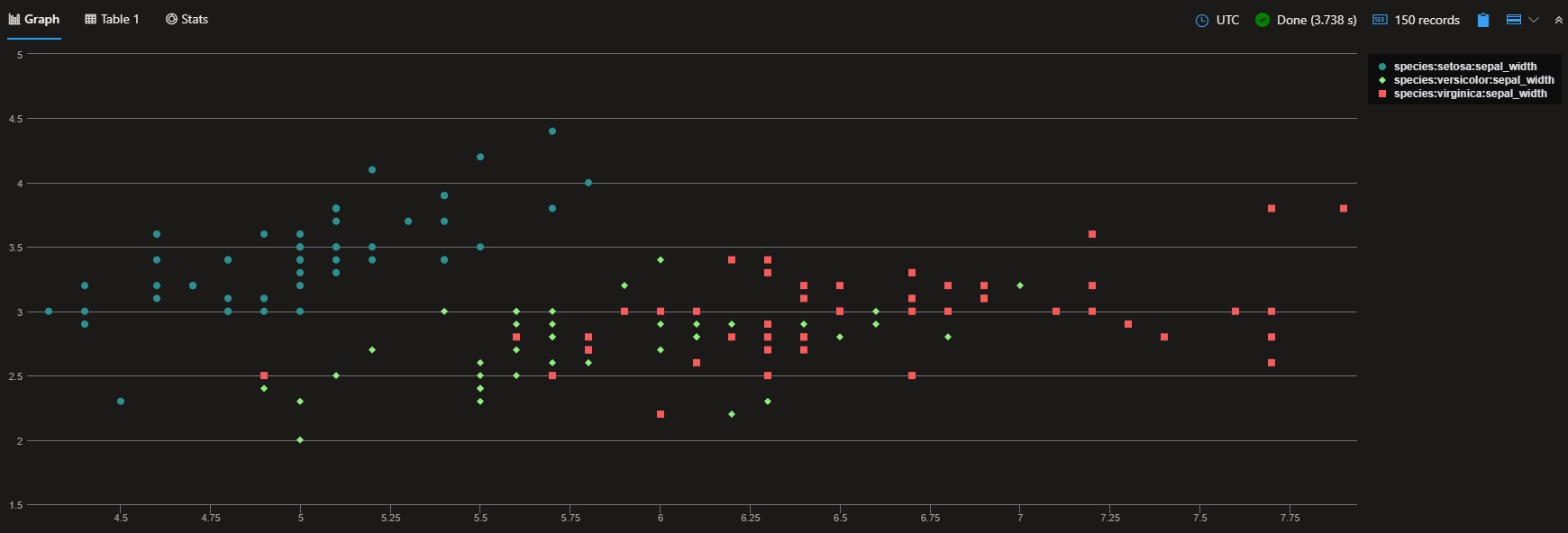
Or perhaps we could plot a scatter chart comparing sepal_width against sepal_length by species:
externaldata(sepal_length:real, sepal_width:real, petal_length:real, petal_width:real, species:string) [
    "https://raw.githubusercontent.com/mwaskom/seaborn-data/master/iris.csv"
]
with(format='csv', ignoreFirstRecord=true)
| render scatterchart with (xcolumn=sepal_length, ycolumns=sepal_width, series=species)
externaldata to retrieve Seaborn Taxi Journey Dataset
Another Seaborn dataset that is interesting to test out is the NYC taxi journey CSV, which is retrieved in a very similar manner (noting different column names/types).
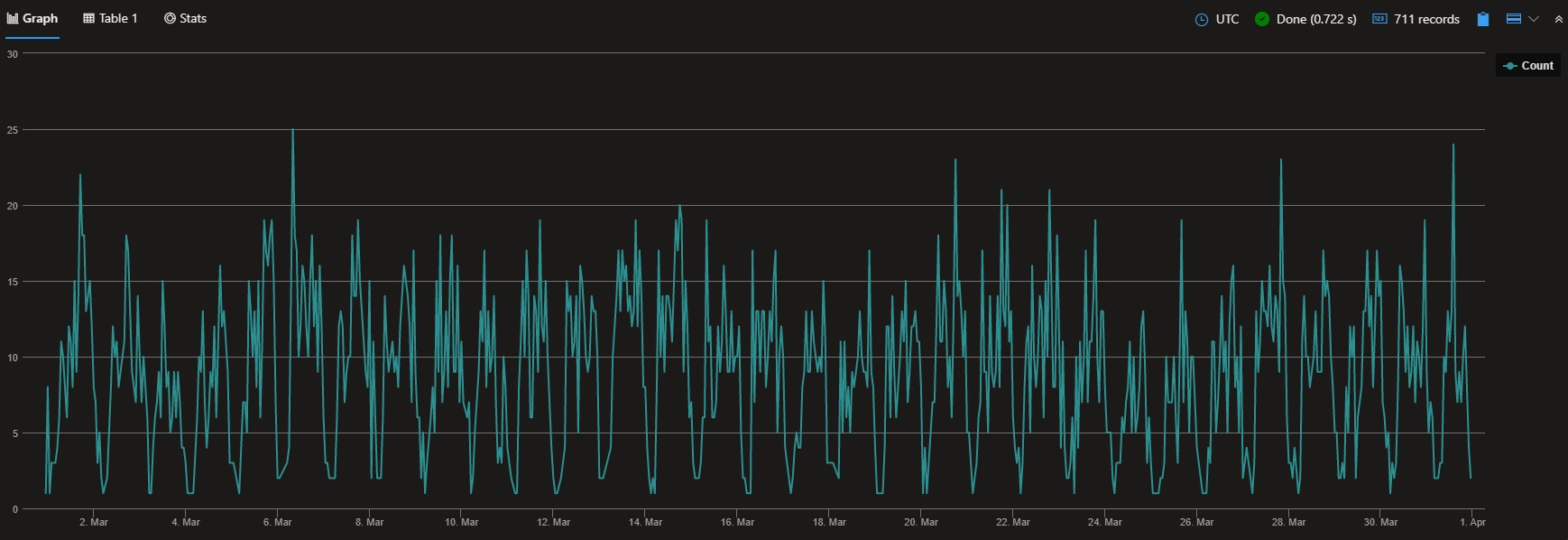
The following query retrieves the data, and draws a quick linechart of journeys per hour:
externaldata(
    pickup:datetime,
    dropoff:datetime,
    passengers:int,
    distance:real,
    fare:real,
    tip:real,
    tolls:real,
    total:real,
    color:string,
    payment:string,
    pickup_zone:string,
    dropoff_zone:string,
    pickup_borough:string,
    dropoff_borough:string
) [
    "https://raw.githubusercontent.com/mwaskom/seaborn-data/master/taxis.csv"
] with(format='csv', ignoreFirstRecord=true)
| summarize Count=count() by bin(pickup, 1h)
| render linechart
Time Series Analysis
KQL has rich support for time series analysis. Here’s a quick query that creates a series out of the above journeys per hour, and then uses the series-periods-detect function to estimate the significant periodic behaviours within the data:
let TaxiData = externaldata(
    pickup:datetime,
    dropoff:datetime,
    passengers:int,
    distance:real,
    fare:real,
    tip:real,
    tolls:real,
    total:real,
    color:string,
    payment:string,
    pickup_zone:string,
    dropoff_zone:string,
    pickup_borough:string,
    dropoff_borough:string
) [
    "https://raw.githubusercontent.com/mwaskom/seaborn-data/master/taxis.csv"
] with(format='csv', ignoreFirstRecord=true)
| project-rename Pickup = pickup;
let PickupStep = 1h;
let PickupMin = toscalar(TaxiData | summarize bin(min(Pickup), PickupStep));
let PickupMax = toscalar(TaxiData | summarize bin(max(Pickup), PickupStep));
TaxiData
| make-series Count = count() on Pickup from PickupMin to PickupMax step PickupStep
| project series_periods_detect(Count, 24 * 0.8, 24 * 7 * 1.2, 2)
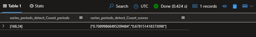
So - the strongest periodic behaviour detected is weekly (168 hours), with a strong daily (24 hour) pattern too.